SOAR, step by step
The Second-Order ARnoldi method of Bai & Su (2005), derived from \(\vZ(\omega)=\vK+\jj\omega\vC-\omega^2\vM\): the expansion, the moments, the second-order Krylov subspace, the SOAR recurrence with deflation and breakdown, the projection, the proofs, and what happens in floating point.
Companion to the lecture Moment Matching Techniques for the Finite Element Method by Pierre Mariotti (KTH). Running example: a 1D impedance tube, small enough to run on any laptop. Every number, curve and reduced model on this page is produced by the open toolbox soar_tube (NumPy/SciPy) with scripts/make_page_data.py, and the raw data is in data/tube/. Section 11 runs the reduced model live in your browser. Section 13 shows the same method on a 3D car cavity.
- Split\(\vZ(\omega_0+\delta)=\vZ_0+\delta\vZ_1+\delta^2\vZ_2\), exactly
- Moments\(\vr_0=\vZ_0^{-1}\vF,\;\; \vr_i=\vA\vr_{i-1}+\vB\vr_{i-2}\)
- Subspace\(\cG_n=\spn\{\vr_0,\dots,\vr_{n-1}\}\), unusable as is
- Basis\(\vH\!\begin{bmatrix}\vQ_n\\\vP_n\end{bmatrix}\!=\!\begin{bmatrix}\vQ_{n+1}\\\vP_{n+1}\end{bmatrix}\!\That_n,\ \vQ_n^{\Hm}\vQ_n=\vI\)
- Project\(\vQ_n^{\Hm}\big(\vK+\jj\omega\vC-\omega^2\vM\big)\vQ_n\,\vy=\vQ_n^{\Hm}\vF\)
- Guarantee\(H_r-H=\mathcal O\big((\omega-\omega_0)^n\big)\); cost: 1 LU + \(n\) solves
The problem and what it costs
A frequency-domain finite element model with frequency-independent matrices, time convention \(e^{\jj\omega t}\), \(\omega=2\pi f\):
\(\vu\in\mathbb C^N\) is the nodal pressure, \(\vF\) the load, and \(H\) a linear output (one row \(\vL^{\Tr}\), no conjugation).
tube_matrices.From the weak form \(\int p'q' + \jj\omega\tfrac{\rho}{Z_s}p(L)q(L)-\omega^2\tfrac1{c^2}\int pq=\rho a\,q(0)\).
- Unknowns (P1, h = 1 mm)N = 1 001
- Band, step20–2000 Hz, 1 Hz
- Frequencies, resonances1 981, 11
- Direct sweep (measured)…
- SOAR to 0.1 % (measured)…
The wall impedance is a dial between a smooth response and sharp resonances (rigid-tube resonances at \(f_n=nc/2L=171.5\,n\) Hz):
| Wall | \(Z_s/\rho c\) | Reflection \(R\) | Peak / valley | Peak width | FE vs exact \(p(L)\) |
|---|
Pressure along the tube
Each frequency of the direct sweep assembles \(\vZ(\omega)\), factorises it and solves. The factorisation has to be redone at every frequency, because \(\vZ\) changes with \(\omega\). Model order reduction replaces \(\vu(\omega)\) by \(\vV\vy(\omega)\) with one frequency-independent basis \(\vV\in\mathbb C^{N\times n}\), \(n\ll N\). Moment matching chooses \(\vV\) from the Taylor expansion of \(\vu\) at one frequency \(\omega_0\). SOAR is a stable way to compute that basis when \(\vZ\) is quadratic.
Four properties of (1.1) are used throughout:
- Quadratic in \(\omega\) with constant matrices. A frequency-dependent impedance \(Z_s(\omega)\) breaks this (Section 12).
- Complex symmetric. \(\vK,\vC,\vM\) are real symmetric, so \(\vZ(\omega)^{\Tr}=\vZ(\omega)\), but \(\vZ^{\Hm}\neq\vZ\).
- \(\vK\vone=\vzero\). No Dirichlet boundary, so \(\vZ(0)=\vK\) is singular: \(\omega=0\) is a pole and \(\omega_0=0\) is not allowed. Physically, an acceleration source has an unbounded static displacement.
- \(\vC\) has one entry. The damping is not proportional (\(\vC\neq\alpha\vK+\beta\vM\)), so the real modes of \((\vK,\vM)\) do not decouple the system. This is the setting where moment matching is the natural tool.
Notation used on this page, and where it lives in the toolbox
| Symbol | Meaning | Size | In soar_tube |
|---|---|---|---|
| \(N,\ n\) | FE unknowns, ROM size | 1 001; 1–40 | K.shape[0], res.n |
| \(\vK,\vC,\vM,\vF,\vL\) | FE arrays and output row | \(N\times N\) sparse, \(N\) | tube_matrices, wall_functional |
| \(\omega_0=2\pi f_0,\ \delta=\omega-\omega_0\) | expansion point, offset | scalars | omega0 |
| \(\vZ_0,\vZ_1,\vZ_2\) | Taylor coefficients of \(\vZ\) at \(\omega_0\) | \(N\times N\) sparse | expansion_matrices |
| \(\vA,\vB\) | \(-\vZ_0^{-1}\vZ_1,\ -\vZ_0^{-1}\vZ_2\): applied, never formed | \(N\times N\) dense | second_order_operator |
| \(\vr_i,\ m_i\) | moments of \(\vu\) and of \(H\) | \(N\), scalar | explicit_moments |
| \(\cG_n(\vA,\vB;\vr_0)\) | second-order Krylov subspace | dim \(n\) | |
| \(\vH\) | \(\begin{bmatrix}\vA&\vB\\\vI&\vzero\end{bmatrix}\), the linearised operator | \(2N\times2N\) | |
| \(\vQ,\ \vP,\ \That\) | SOAR vectors, auxiliary vectors, coefficients | \(N\times m\), \(m\times(m-1)\) | SoarResult.Q, .P, .T |
| \(\vV\) | reduced basis: the non-zero columns of \(\vQ\) | \(N\times n\) | soar_basis(...).V |
| \(\vK_r,\vC_r,\vM_r,\vF_r,\vL_r\) | reduced arrays | \(n\times n\), \(n\) | project |
Expanding \(\vZ(\omega)\) around \(\omega_0\)
Put \(\omega=\omega_0+\delta\) and expand:
- The split is exact. \(\vZ\) is a polynomial of degree 2, so \(\vZ_1=\vZ'(\omega_0)\), \(\vZ_2=\tfrac12\vZ''(\omega_0)\) and no term is dropped.
- Only \(\vZ_0\) is factorised. \(\vZ_1\) and \(\vZ_2\) are only multiplied with vectors.
- \(\vZ_0\) must be invertible, so \(\omega_0\) must not be a pole. All poles of the tube satisfy \(\mathrm{Im}\,\omega\ge0\) (Section 8), and the only real one is \(\omega=0\) (Section 3). Any real \(\omega_0>0\) therefore works in exact arithmetic. Near a lightly damped resonance \(\vZ_0\) is close to singular, but sparse LU with pivoting stays backward stable.
# soar_tube/moments.py and soar_tube/fom.py
Z0, Z1, Z2 = expansion_matrices(K, C, M, omega0)   # K + 1j*omega0*C - omega0**2*M,  1j*C - 2*omega0*M,  -M
solve0 = lu_solver(Z0)                            # one sparse LU (SciPy SuperLU), returns solve(b)
Moments: the Taylor coefficients of \(\vu\)
Because \(\vZ_0\) is invertible, \(\vu(\omega)=\vZ(\omega)^{-1}\vF\) is analytic in a disk around \(\omega_0\). Its radius \(\rho\) is the distance from \(\omega_0\) to the nearest pole, i.e. the nearest root of \(\det\vZ(\omega)=0\):
Insert (2.1) and (3.1) into \(\vZ\vu=\vF\) and collect equal powers of \(\delta\):
Hence the three-term recurrence that defines everything that follows:
Each new moment costs two sparse products and one forward and backward substitution with the LU factors of \(\vZ_0\). \(\vA\) and \(\vB\) are dense and are never formed. The output moments are \(m_i=\vL^{\Tr}\vr_i\), so \(H(\omega_0+\delta)=\sum_i m_i\delta^i\).
The Taylor series converges only in a small disk
The tube's poles are known in closed form. With \(R=(Z_s-\rho c)/(Z_s+\rho c)\), \(\det\vZ=0\) for the continuous problem when \(R\,e^{-2\jj kL}=1\):
all with the same damping (analytic_poles_hz). The FE poles agree to …. For the moderate wall, the pole nearest to \(f_0=1040\) Hz is at …. So (3.1) converges only within … of 1040 Hz, i.e. on …. Yet the SOAR model with 20 vectors is accurate to 0.1 % over 20–2000 Hz. A reduced model is not a truncated Taylor series. It is a rational function whose poles move towards the true poles (Section 8). This is the main conceptual point of moment matching.
Poles of \(H(\omega)\) near the band, moderate wall
\(\vK\vone=\vzero\) makes \(\omega=0\) an exact pole. The \(n=0\) pole of (3.3) lies on the imaginary axis. The Rayleigh quotient of \(\vZ\) on the constant mode estimates it:
which gives \(f_c=\)…, against … from (3.3). This pair produces the low-frequency rise of the response.
Why not use the moments directly
Asymptotic waveform evaluation (AWE, Pillage & Rohrer 1990) builds a Padé approximant from the scalar moments \(m_i\). One could also project on \(\spn\{\vr_0,\dots,\vr_{n-1}\}\) computed with (3.2). Both fail after a handful of moments in double precision (… on the tube). The reason is that (3.2) is a power iteration.
Let \(\vZ(\omega_p)\vx=\vzero\), \(\omega_p=\omega_0+\delta_p\). Then \((\vZ_0+\delta_p\vZ_1+\delta_p^2\vZ_2)\vx=\vzero\). Multiply by \(-\vZ_0^{-1}/\delta_p^2\) and set \(\mu=1/\delta_p\):
So every pole \(\omega_p\) gives an eigenvalue \(\mu=1/(\omega_p-\omega_0)\) of \(\vH\). Written for pairs of moments, (3.2) is
This is the power method on \(\vH\). The normalised moments turn towards the eigenvectors with the largest \(|\mu|\), i.e. the poles closest to \(\omega_0\), and each new moment adds less and less new direction. Scaling does not help: it cures the growth of \(\|\vr_i\|\sim\rho^{-i}\), not the loss of direction.
New direction in each explicit moment, \(f_0=1040\) Hz
new_direction). The moments are scaled by \(\rho^i\) to avoid overflow. After … moments the new direction is at round-off level.ROM error against \(n\), \(f_0=1040\) Hz, output \(p(L)\)
An orthonormal basis of \(\spn\{\vr_0,\dots,\vr_{n-1}\}\), built without forming the moments. For a linear operator, Arnoldi does exactly that. The next two sections build the second-order version.
The second-order Krylov subspace and its linearisation
Definition (Bai & Su 2005). For \(\vA,\vB\in\mathbb C^{N\times N}\) and \(\vr_0\neq\vzero\):
With \(\vA,\vB,\vr_0\) from (3.2), \(\cG_n\) is exactly the span of the first \(n\) moments of \(\vu\). For \(\vB=\vzero\) it reduces to the ordinary Krylov subspace \(\cK_n(\vA;\vr_0)\).
Linearisation. Stack two consecutive moments, \(\vw_i=\begin{bmatrix}\vr_i\\\vr_{i-1}\end{bmatrix}\in\mathbb C^{2N}\). The top block of \(\vH\vw_{i-1}\) is \(\vA\vr_{i-1}+\vB\vr_{i-2}=\vr_i\), and the bottom block is \(\vr_{i-1}\). So
The second-order Krylov subspace is the top half of an ordinary Krylov subspace of dimension \(2N\). By (4.1), the eigenvalues of \(\vH\) are \(\mu=1/(\omega_p-\omega_0)\). \(\vH\) is the shift-and-invert operator of a companion linearisation, which is why Krylov methods on \(\vH\) find the poles nearest \(\omega_0\) first.
This gives two routes:
- Route A, linearise then reduce. Arnoldi on \(\vH\) gives an orthonormal \(\vV_n\in\mathbb C^{2N\times n}\). The vectors are twice as long, so memory and Gram–Schmidt cost double. The top block spans \(\cG_n\) but is not orthonormal and must be re-orthonormalised. Projecting the first-order (linearised) system instead gives a first-order ROM that loses the \(\vK,\vC,\vM\) structure and the stability argument of Section 8.
- Route B, SOAR. Orthonormalise only the top block. Carry the bottom block as auxiliary vectors \(\vp_j\) of length \(N\). Never form a vector of length \(2N\).
Deriving the SOAR recurrence
Goal. Build \(\vQ_n=[\vq_1,\dots,\vq_n]\) with \(\vQ_n^{\Hm}\vQ_n=\vI\) and \(\spn\{\vq_1,\dots,\vq_j\}=\cG_j\) for every \(j\le n\), using vectors of length \(N\) only.
Ansatz (Bai & Su). Look for auxiliary vectors \(\vP_n=[\vp_1,\dots,\vp_n]\) and an \((n+1)\times n\) upper Hessenberg matrix \(\That_n=(t_{ij})\) such that the stacked vectors satisfy an Arnoldi-type relation with \(\vH\):
The difference with Arnoldi is that only the top block \(\vQ\) is required to be orthonormal. Write (6.1) block row by block row:
Column \(j\) of the top equation. \(\vA\vq_j+\vB\vp_j=\sum_{i=1}^{j+1}\vq_i\,t_{ij}\). Multiply by \(\vq_k^{\Hm}\), \(k\le j\), and use orthonormality:
This is Gram–Schmidt of the candidate \(\vA\vq_j+\vB\vp_j\) against \(\vQ_j\).
Column \(j\) of the bottom equation. \(\vq_j=\sum_{i=1}^{j+1}\vp_i\,t_{ij}\), so
The bottom block is not orthogonalised. It receives the same coefficients \(t_{ij}\), because (6.1) requires it. Start: \(\vw_0=[\vr_0;\vzero]\) scaled by \(1/\|\vr_0\|\), so \(\vq_1=\vr_0/\|\vr_0\|\) and \(\vp_1=\vzero\).
Meaning of \(\vp_j\). The recurrence \(\vr_i=\vA\vr_{i-1}+\vB\vr_{i-2}\) needs two vectors, the current moment and the previous one. SOAR does the same with \(\vq_j\) and its companion \(\vp_j\), which stands for "the previous vector" in the stacked pair \([\vr_i;\vr_{i-1}]\).
If \(t_{k+1,k}\neq0\) for \(k=1,\dots,j-1\), then \(\spn\begin{bmatrix}\vQ_j\\\vP_j\end{bmatrix}=\cK_j(\vH;\vw_0)\) and \(\spn\vQ_j=\cG_j(\vA,\vB;\vr_0)\).
Since \(\vp_1=\vzero\), the first row of \(\That_n\) drops out of the bottom equation \(\vQ_n=\vP_{n+1}\That_n\):
\(\Ts\) is upper triangular with the non-zero subdiagonal entries of \(\That_n\) on its diagonal, so it is invertible and
- \(\vp_{j+1}\in\spn\{\vq_1,\dots,\vq_j\}\). The projection basis is \(\vQ\) alone.
- \(\vP\) need not be stored. Bai & Su's memory-saving variant recomputes \(\vp_j\) from \(\vQ\) and \(\That\), which needs \(Nn\) storage instead of \(2Nn\).
- The norm of \(\vp_{j+1}\) is exactly that of a column of \(\Ts^{-1}\). If \(\Ts\) is ill-conditioned, the auxiliary vectors grow (Section 9).
Check on the tube (moderate wall, \(f_0=1040\) Hz, the … steps before the first deflation): \(\|[\vp_2,\dots]-\vQ\Ts^{-1}\|/\|[\vp_2,\dots]\|=\)….
Taking the first \(n\) rows of \(\That_n\) as \(\vT_n\), (6.1) reads
the analogue of the Arnoldi decomposition. Bai & Su introduced SOAR for the quadratic eigenvalue problem. For eigenvalues they project the QEP onto \(\vQ_n\) (Rayleigh–Ritz) rather than using \(\vT_n\). The reduced model of Section 8 is that same projection.
The algorithm, with deflation and breakdown
If \(t_{j+1,j}=0\) in (6.4), the candidate brings no new direction to the top block and the recurrence cannot divide by it. Bai & Su's Algorithm 2 separates two cases:
- Deflation. \(\vA\vq_j+\vB\vp_j\in\spn\vQ_j\), but the stacked vector \([\vzero;\vs]\) is still new. Set \(t_{j+1,j}=1\), \(\vq_{j+1}=\vzero\), \(\vp_{j+1}=\vs\), and continue. \(\cG\) pauses while \(\cK(\vH;\vw_0)\) keeps growing, and later steps can bring new directions back into the top block. The zero columns of \(\vQ\) are dropped at the end.
- Breakdown. If also \(\vs\in\spn\{\vp_i:\ \vq_i=\vzero\}\), then \(\cK_j(\vH;\vw_0)\) is invariant under \(\vH\). Every moment lies in \(\cG_j\), so \(\vu(\omega)\in\cG_j\) on the Taylor disk, and by analytic continuation for all \(\omega\). In exact arithmetic the ROM is then exact (a "lucky" breakdown) and the procedure stops.
soar_basis, soar_iterate · input \(\vK,\vC,\vM,\vF,\omega_0,n\); tol = \(10^{-12}\), reorth = 2, at most \(2n\) steps| 1 | \(\vZ_0\leftarrow\vK+\jj\omega_0\vC-\omega_0^2\vM\); factorise \(\vZ_0=\mathbf{LU}\) | one sparse LU · … |
| 2 | \(\vZ_1\leftarrow\jj\vC-2\omega_0\vM\); \(\vZ_2\leftarrow-\vM\) | |
| 3 | \(\vr_0\leftarrow\vZ_0^{-1}\vF\); \(\vq_1\leftarrow\vr_0/\|\vr_0\|\); \(\vp_1\leftarrow\vzero\); \(\mathcal D\leftarrow\varnothing\) ▹ \(\mathcal D\): indices of zero \(\vq\) columns | one substitution |
| 4 | for \(j=1,2,\dots\) while (number of non-zero \(\vq\)) \(<n\) | |
| 5 | \(\vr\leftarrow-\vZ_0^{-1}\big(\vZ_1\vq_j+\vZ_2\vp_j\big)\); \(\vs\leftarrow\vq_j\); \(\eta\leftarrow\|\vr\|\) ▹ \(\vr=\vA\vq_j+\vB\vp_j\) | 2 sparse products + 1 substitution |
| 6 | repeat twice: \(\vh\leftarrow\vQ_j^{\Hm}\vr\); \(\vr\leftarrow\vr-\vQ_j\vh\); \(\vs\leftarrow\vs-\vP_j\vh\); \(t_{1:j,j}\mathrel{+}=\vh\) ▹ CGS2, same \(\vh\) for both blocks | \(3Nj\) |
| 7 | if \(\|\vr\|>\text{tol}\cdot\eta\): \(t_{j+1,j}\leftarrow\|\vr\|\); \(\vq_{j+1}\leftarrow\vr/\|\vr\|\); \(\vp_{j+1}\leftarrow\vs/\|\vr\|\) ▹ normal step | … per step |
| 8 | else if \(\vs\notin\spn\{\vp_i: i\in\mathcal D\}\): \(t_{j+1,j}\leftarrow1\); \(\vq_{j+1}\leftarrow\vzero\); \(\vp_{j+1}\leftarrow\vs\); \(\mathcal D\leftarrow\mathcal D\cup\{j+1\}\) ▹ deflation | small least squares |
| 9 | if the last three steps were deflations: stop ▹ numerical stagnation; an addition to Alg. 2 (max_consecutive_deflations) | |
| 10 | else: stop ▹ breakdown: \(\cK_j(\vH;\vw_0)\) is invariant | |
| 11 | \(\vV\leftarrow[\vq_i:\ i\notin\mathcal D]\) ▹ the reduced basis |
# the loop of soar_iterate() in soar_tube/soar.py, lines 4-10 of the algorithm
while n_basis < n and j < max_steps:
    r = apply(Q[:, j], P[:, j])                    # r = A q_j + B p_j  (one back-substitution)
    s = Q[:, j].copy()                             # s = q_j
    eta = np.linalg.norm(r)
    r, s, h = gram_schmidt_qp(Q[:, : j + 1], P[:, : j + 1], r, s, reorth)
    T[: j + 1, j] = h
    beta = np.linalg.norm(r)
    if beta > tol * eta:                           # normal step
        T[j + 1, j] = beta
        Q[:, j + 1] = r / beta
        P[:, j + 1] = s / beta
        n_basis += 1
        run = 0                                    # consecutive deflations
    else:
        scale = max(np.linalg.norm(Q[:, j]), np.linalg.norm(P[:, : j + 1] @ h))
        if in_span(s, P[:, zero_cols], tol, scale):  # breakdown: invariant subspace
            breakdown, breakdown_step = True, j + 1
            break
        T[j + 1, j] = 1.0                          # deflation: q_{j+1} = 0, continue
        Q[:, j + 1] = 0.0
        P[:, j + 1] = s
        zero_cols.append(j + 1)
        run += 1
        if run >= max_consecutive_deflations:     # default 3: numerical stagnation
            break
    j += 1
With a single load vector on an FE model, exact deflation does not occur in practice. Both branches are therefore tested on small matrices built to trigger them (tests/test_soar_tube.py): if \(\vA\vu=\lambda\vu\), SOAR deflates at step 1 and continues with \(\vB\vu\); if moreover \(\vB\vu=\mu\vu\), the subspace is \(\spn\{\vu\}\) and SOAR breaks down at step 2. In floating point, line 8 can also fire for a numerical reason, which Section 9 shows on the tube.
Projection, moment matching and stability
Approximate \(\vu(\omega)\approx\vV\vy(\omega)\) and ask the residual to be orthogonal to \(\spn\vV\) (Galerkin): \(\vV^{\Hm}\big(\vF-\vZ(\omega)\vV\vy\big)=\vzero\). This gives
and \(H_r(\omega)=\vL_r^{\Tr}\vy(\omega)\) with \(\vL_r^{\Tr}=\vL^{\Tr}\vV\) (project, rom_solve, rom_sweep).
- Same structure. The ROM is quadratic in \(\omega\) with constant \(n\times n\) matrices: \(\mathcal O(n^3)\) per frequency and no reassembly.
- Nested. \(\vV_k\) is the first \(k\) columns of \(\vV_n\). The size-\(k\) ROM is therefore the leading \(k\times k\) block of (8.1): one projection serves every size (
truncate). - Only the subspace matters. Replacing \(\vV\) by \(\vV\vS\) (\(\vS\) invertible) changes \(\vy\) to \(\vS^{-1}\vy\) and leaves \(H_r\) unchanged. In exact arithmetic, SOAR, Arnoldi on \(\vH\) with a QR of the top block, the explicit-moment basis and WCAWE (for this quadratic \(\vZ\)) all give the same ROM. They differ only in floating point.
- The basis depends on \(\vF\), not on \(\vL\). One basis serves every output: the wall pressure and the space-averaged pressure need the same \(n\) (Section 10).
Let \(\vV\in\mathbb C^{N\times n}\), \(\vV^{\Hm}\vV=\vI\), \(\cG_n(\vA,\vB;\vr_0)\subseteq\spn\vV\), and let \(\vZ_{r,0}=\vV^{\Hm}\vZ_0\vV\) be invertible. Let \(\boldsymbol\rho_i\) be the moments of the ROM (8.1) built with \(\vV\). Then \(\vV\boldsymbol\rho_i=\vr_i\) for \(i=0,\dots,n-1\), so
The proof only uses \(\cG_n\subseteq\spn\vV\). The job of SOAR is to deliver that subspace with an orthonormal, well-conditioned basis.
If \(\vK,\vC,\vM\) are complex symmetric (true for the tube) and \(\vL=\alpha\vF\), use the transpose instead of the conjugate transpose: \(\vZ_r=\vV^{\Tr}\vZ\vV\), \(\vF_r=\vV^{\Tr}\vF\). Then \(H-H_r=\mathcal O\big((\omega-\omega_0)^{2n}\big)\).
The price: \(\vV^{\Tr}\vM\vV\) is not Hermitian, so Theorem 8.3 below no longer applies. On the tube \(\vF=\rho a\,\ve_1\), so \(\vL\propto\vF\) is the pressure on the piston, \(p(0)\): a driving-point quantity, directly related to the input impedance.
Checking the orders on the tube: error near \(f_0=1040\) Hz, output \(p(0)\) on the piston
Assume \(\vK=\vK^{\Hm}\succeq0\), \(\vM=\vM^{\Hm}\succ0\) and \(\vC+\vC^{\Hm}\succeq0\) (passive walls). Then every pole of the full model and of the ROM (8.1), for any full-rank \(\vV\), satisfies \(\mathrm{Im}\,\omega_p\ge0\). With \(e^{\jj\omega t}\), no free response grows.
Tube: \(\vK,\vM\) real symmetric, \(\vC=\frac{\rho}{Z_s}\ve_N\ve_N^{\Tr}\succeq0\) for any \(Z_s>0\). Checked over the three walls, the seven expansion points of the demo and every \(n\) (… ROM poles, rom_poles_hz): \(\min\mathrm{Im}\,f_p=\)…, round-off around the exact pole at 0. The congruence \(\vV^{\Hm}(\cdot)\vV\) is what preserves the property. \(\vV^{\Tr}\) and first-order ROMs of the linearisation do not have it.
What kind of approximant is \(H_r\)?
\(\det\vZ_r(\omega)\) is a polynomial of degree \(2n\), so \(H_r\) is rational with \(2n\) poles and a numerator of degree at most \(2n-2\). A Padé approximant with that many poles would match about \(4n\) moments. The one-sided ROM matches \(n\), the two-sided one \(2n\), and the rest of the freedom goes to keeping \(\vK,\vC,\vM\) and stability. The ROM poles lock onto the true poles nearest \(\omega_0\) first, so the accurate band grows outward from \(f_0\) as \(n\) increases. The live demo shows this.
What happens in floating point
Orthogonality
Classical Gram–Schmidt applied twice (CGS2, "twice is enough") keeps \(\vV\) orthonormal to working precision: \(\|\vV^{\Hm}\vV-\vI\|=\)… at 1040 Hz (moderate wall), and the recurrence (6.1) holds to … (check_basis, soar_relation_residual). A single CGS pass loses orthogonality as the basis converges.
The auxiliary vectors grow
By (6.7), \(\|\vp_{j+1}\|=\|\Ts^{-1}\ve_j\|\). The diagonal of \(\Ts\) holds the subdiagonal entries \(t_{k+1,k}\), the size of each new direction. As the subspace captures the poles near \(\omega_0\), these entries shrink relative to the other \(t_{ik}\). This is the same mechanism that makes the Arnoldi subdiagonal shrink when Ritz values converge. \(\Ts^{-1}\) then grows geometrically.
The consequence: the candidate \(\vA\vq_j+\vB\vp_j\) is dominated by \(\vB\vp_j\), and that part lies almost entirely in \(\spn\vQ_j\). Gram–Schmidt removes it. What remains is the fraction
of the candidate. A rounding error of order \(\varepsilon\|\vA\vq_j+\vB\vp_j\|\) in the candidate becomes a relative error of about \(\varepsilon/\eta_j\) in \(\vq_{j+1}\). When \(\eta_j\) reaches the tolerance \(10^{-12}\), line 7 of the algorithm declares a deflation: the new direction is indistinguishable from round-off.
Norm of the auxiliary vectors \(\|\vp_j\|\)
New fraction of each candidate, \(\eta_j\)
Moderate wall, three expansion points, every step of the algorithm (normal steps and deflations). Dashed line: \(\eta=10^{-12}\). …
Numerical deflations, then SOAR stops
On the tube, every run of 40 vectors ends the same way. Once \(\|\vp_j\|\) reaches \(10^{14}\)–\(10^{16}\), \(\eta_j\) falls below the tolerance, line 8 deflates, and the following candidates are dominated by round-off as well. Left alone, the deflations would come in a cascade until the span test declares a breakdown, without adding a single vector; soar_basis therefore stops after three deflations in a row (line 9, stopped_reason = "deflations"). The basis then stops growing. These are numerical events, not the exact deflation of Section 7, and they decide how far SOAR can go:
- At a good expansion point it does no harm. At 1040 Hz the basis stops at … vectors, when the error is already ….
- Far from part of the band it does. At 200 Hz, at the edge of a 20–2000 Hz band, the basis stops at … vectors with a … error. A stable basis of the same subspace (Arnoldi on the \(2N\) linearisation, then QR of the top block) keeps converging, below. The stall is a precision effect, not a property of the subspace.
Same subspace, two bases: SOAR against Arnoldi on the linearisation, \(f_0=200\) Hz, moderate wall
Rescaling \(\omega\) does not help. With \(\delta=s\delta'\): \(\vA\to s\vA\), \(\vB\to s^2\vB\), every \(\vp_j\to\vp_j/s\) and every \(t_{ij}\to s\,t_{ij}\). \(\eta_j\) does not change. The cause is structural: SOAR normalises the top block only, so it divides by \(t_{j+1,j}\) even when the stacked vector \([\vq;\vp]\) still carries plenty of new information. TOAR (Section 12) normalises the whole stacked vector and avoids the division.
In practice: always use CGS2, monitor \(\eta_j\), \(\|\vp_j\|\) and the deflations reported by soar_basis, and when they appear before the error is small enough, either switch to TOAR or add a second expansion point instead of pushing \(n\).
Choosing \(\omega_0\), \(n\), the output and the number of points
Where to expand
The tube's modes are evenly spaced (171.5 Hz apart), so the best expansion point sits near the middle of the band: …. Moving away costs vectors on the far side, and far below the centre SOAR stops before reaching 0.1 % (…; Section 9).
In a 3D cavity the modes get denser with frequency, and the best point moves to where they are dense: the median mode rather than the band centre (Section 13).
Vectors needed for 0.1 % against \(f_0\), output \(p(L)\)
Which output
The basis depends on \(\vF\), not on the output. The space-averaged pressure \(\overline{p}^{\,2}=\frac1L\int_0^L|p|^2\,\mathrm dx=\frac{c^2}{L}\vu^{\Hm}\vM\vu\), a smooth "engineering" metric, is quadratic: its moments are not matched literally, but in the ROM it costs \(\frac{c^2}{L}\vy^{\Hm}\vM_r\vy\), independent of \(N\) (mean_square_pressure). It needs the same \(n\) as \(p(L)\): ….
Error against \(n\) for two outputs of the same ROM, moderate wall, \(f_0=1040\) Hz
How many vectors, without the full model
- Nested difference. All sizes \(k\le n\) come for free (leading blocks), so \(\|H_n-H_{n-d}\|/\|H_n\|\) over the band (\(d=2\) to 5) is a free error indicator. Stop when it falls below the tolerance.
- Residual at \(\mathcal O(n^2)\) per frequency. \(\vR(\omega)=\vF-\vZ(\omega)\vV\vy=\vW\vc(\omega)\) with \(\vW=[\vF,\ \vK\vV,\ \vC\vV,\ \vM\vV]\) and \(\vc=[1;\,-\vy;\,-\jj\omega\vy;\,\omega^2\vy]\). Precompute \(\vG=\vW^{\Hm}\vW\) once (size \(3n+1\)); then \(\|\vR(\omega)\|^2=\vc^{\Hm}\vG\vc\) costs nothing that depends on \(N\). Since error \(\le\|\vZ(\omega)^{-1}\|\,\|\vR(\omega)\|\), a small residual can still hide a large error at a lightly damped peak.
- Rule of thumb: about two vectors per mode in the band (tube: 11 resonances, \(n\approx19\)–20 for \(10^{-3}\); car of Section 13: 8 modes, \(n\approx20\)).
One point or several
Multi-point SOAR concatenates the bases built at several \(\omega_k\), orthonormalises them and projects once (multipoint_basis, union_basis). Theorem 8.1 applies at every \(\omega_k\), because each \(\cG_{n_k}(\omega_k)\) lies in the union. Each point costs one LU. Counted in units of one SOAR vector, with \(\beta\) = cost of one LU / cost of one vector:
| Configuration | LUs | Vectors for 0.1 % | Vectors for \(10^{-6}\) | Cost, \(\beta\) = 2 (tube) | Cost, \(\beta\) = 72 (3D car) |
|---|
Extra points save one or two vectors on the tube, because one point already covers the band. With \(\beta\approx2\) in 1D that is a wash; with \(\beta\approx72\) on a 3D model it is a clear loss. An extra point pays only if it saves more vectors than one LU costs, or if the factorisations run in parallel.
Where the time goes
… In 1D a sparse LU costs about as much as a back-substitution, so the speed-up is modest. When the LU dominates, as in 3D, the speed-up approaches the number of frequencies: the whole SOAR model costs about as much as one frequency of the direct sweep (Section 13).
The online stage, live
The SOAR bases (1 001 × up to 40 per expansion point) were computed offline by soar_basis. This page holds only what the online stage needs: the Hermitian matrices \(\vK_r\), \(\vC_r\), \(\vM_r\) and the vectors \(\vF_r\), \(\vL_r\), for three walls and seven expansion points. Every change below solves (8.1) in your browser at the 1 981 frequencies, as rom_sweep does. The full-model reference is the direct sweep.
- Relative \(L^2\) error…
- Max level error…
- Within 1 dB around \(f_0\)…
- Taylor radius at \(f_0\)…
- Basis size reached…
- ROM sweep, 1 981 frequencies…
Sound pressure level on the wall, full model against ROM
Level error \(|L_{\text{ROM}}-L_{\text{FOM}}|\)
Relative error against \(n\) at this \(f_0\)
Poles: ROM (\(2n\)) and full model
Things to try: at \(f_0=1040\) Hz, step \(n\) from 5 to 20 and watch the 1-dB band and the captured poles grow outward from \(f_0\). Switch to the strong wall: the peaks are 2.8 Hz wide and 32 dB high, yet \(n\approx20\) still suffices. Move \(f_0\) to 200 Hz: the basis stops early (Section 9). The matched wall has no resonance but still needs about 19 vectors: \(n\) follows the number of half-wavelengths in the band, not the peaks.
Beyond SOAR
| Method | Vectors stored | Orthonormal | ROM keeps \(\vK,\vC,\vM\) | Finite precision | Scope |
|---|---|---|---|---|---|
| Explicit moments (AWE) | \(N\) | no | if projected | collapses after a few moments | any polynomial \(\vZ\) |
| Arnoldi on \(\vH\) | \(2N\) | stacked vectors | only after extracting the top block | stable | any polynomial \(\vZ\) |
| SOAR | \(N\) (+\(N\) auxiliary) | \(\vQ\) only | yes | auxiliary vectors can grow | quadratic \(\vZ\) |
| TOAR | \(N\) + small coefficients | stacked vectors | yes | backward stable (Lu, Su & Bai 2016) | polynomial \(\vZ\) |
| WCAWE | \(N\) | yes | yes | stable in practice | general \(\vZ(\omega)=\sum_k f_k(\omega)\vZ_k\) |
TOAR in a few lines
The bottom block of \(\vH\vv\) is the top block of \(\vv\). So every block of every Arnoldi vector of \(\cK_j(\vH;\vw_0)\) lies in \(\cG_{j+1}=\spn\{\vr_0,\dots,\vr_j\}\). Write the orthonormal Arnoldi basis as
One step computes \(\vr=\vA(\vU\vs_1)+\vB(\vU\vs_2)\) (one substitution), orthogonalises \(\vr\) against \(\vU\) (first level, length \(N\)), and then orthogonalises the new coordinate vector against \(\vS\) (second level, small). Memory is about \(N(n+1)\), like SOAR. The stacked basis is orthonormal, like Arnoldi on \(\vH\), so nothing is divided by a small top-block norm. The subspace and the ROM are the same as SOAR's. TOAR is available in SLEPc (PEPTOAR, Campos & Roman 2016) and extends to higher-degree polynomials (Kressner & Roman 2014).
Other directions
- Frequency-dependent load. For \(\vF(\omega_0+\delta)=\sum_k\vF_k\delta^k\), the recurrence becomes \(\vZ_0\vr_i=\vF_i-\vZ_1\vr_{i-1}-\vZ_2\vr_{i-2}\). For a velocity source \(\jj\omega\rho\,v\), it is simpler to solve with the constant part and multiply the output by \(\jj\omega\) (the problem is linear). This is why the tube is driven by an acceleration.
- Frequency-dependent impedance or admittance. \(\vZ\) is no longer quadratic. Use WCAWE (Souza Lenzi et al. 2013, §6.1.2), or fit a rational impedance and add auxiliary unknowns to recover a polynomial system.
- Several loads. Block SOAR with \(\vF=[\vF_1,\dots,\vF_m]\).
- Two-sided projection. \(2n\) moments with a second, output-dependent subspace (Theorem 8.2 is the symmetric special case).
- Eigenvalues. SOAR was designed for the QEP. Rayleigh–Ritz on \(\vV\) gives the ROM poles shown in the demo.
Same method at scale: a car cavity
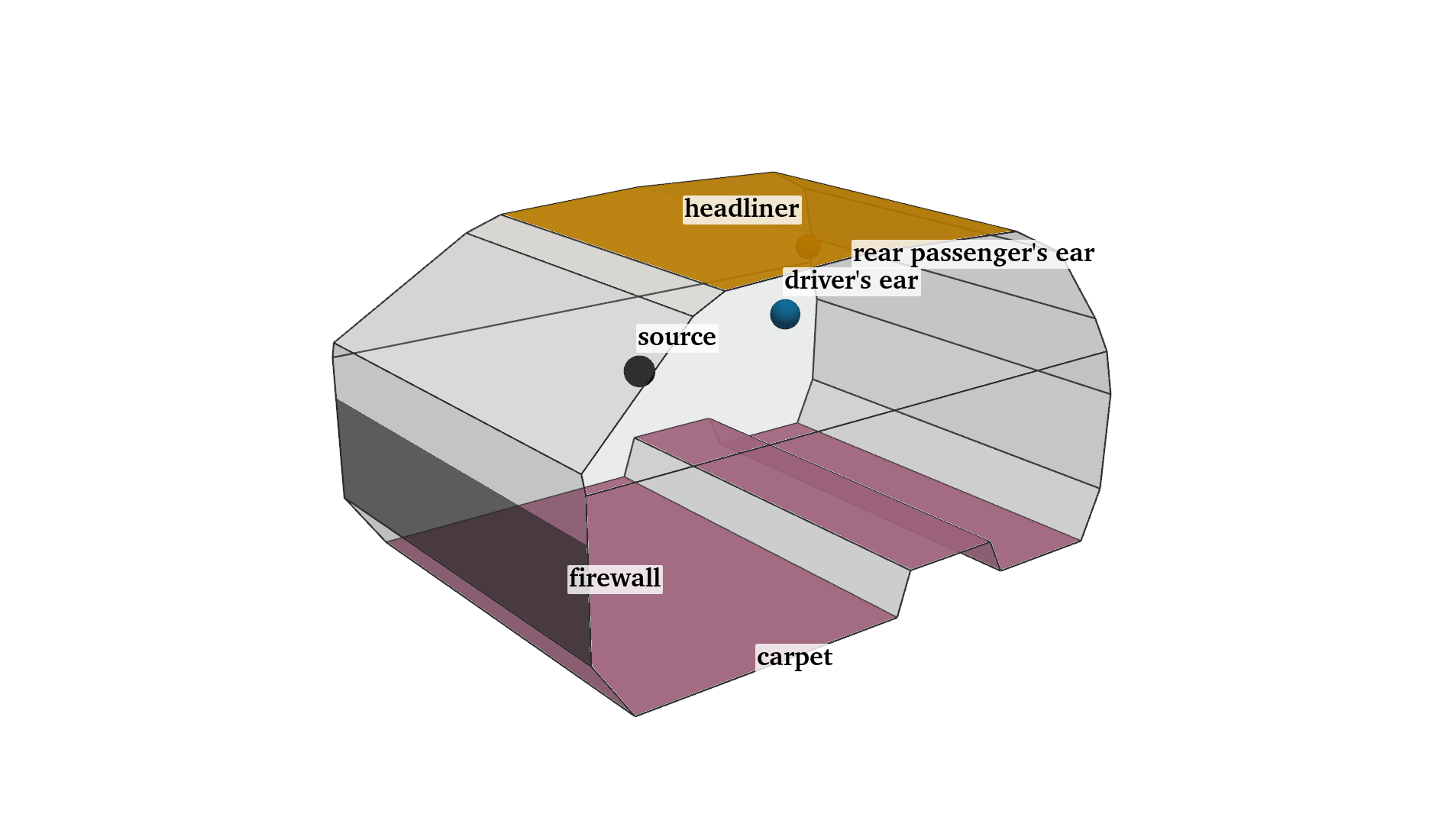
The lecture applies exactly the same algorithm to a 3D cavity, where the full model is large enough for the factorisation to dominate.
- Physics. Helmholtz equation, \(c=340\) m/s, \(\rho=1.225\) kg/m³. Rigid walls, except a constant normalised admittance \(\bar A=\rho c A=6.8\cdot10^{-3}+6.9\cdot10^{-2}\,\jj\) on the headliner and the carpet. Unit point source \(-4\pi\delta(\mathbf x-\mathbf x_s)\), \(\mathbf x_s=(0.5,\,0.45,\,0.9)\) m. Band 10–200 Hz (8 cavity modes).
- Matrices. \(K_{ij}=\int\nabla\varphi_i\cdot\nabla\varphi_j\), \(M_{ij}=\frac1{c^2}\int\varphi_i\varphi_j\), \(C_{ij}=\frac{\bar A}{c}\int_{\Gamma_a}\varphi_i\varphi_j\) (complex, boundary-only), \(F_i=-4\pi\varphi_i(\mathbf x_s)\): the same \(\vZ(\omega)=\vK+\jj\omega\vC-\omega^2\vM\).
- Numbers from the lecture (P2, 65 515 dofs, 191 frequencies, single core, MUMPS, \(f_0=105\) Hz): direct sweep 1 096 s; SOAR with \(n=20\) (1 % at the driver's ear) 7.4 s, ×148. One LU costs as much as about 72 SOAR vectors.
The repository provides the car case without any FE code:
data/car_cavity/car_cavity.md: geometry, boundary conditions, parameters and what was assumed.car_cavity.step: the cavity solid (any CAD tool or gmsh);car_cavity_geometry.py: the gmsh script that builds and labels it.car_cavity_p2_19072dofs.npz: assembled \(\vK,\vC,\vM,\vF\) and the ear outputs of a converged 19 072-dof P2 model, ready forsoar_basis;examples/05_car_cavity.pyruns SOAR on it.
References
- Z. Bai, Y. Su. SOAR: A second-order Arnoldi method for the solution of the quadratic eigenvalue problem. SIAM J. Matrix Anal. Appl. 26(3), 640–659, 2005.
- Z. Bai, Y. Su. Dimension reduction of large-scale second-order dynamical systems via a second-order Arnoldi method. SIAM J. Sci. Comput. 26(5), 1692–1709, 2005.
- M. Souza Lenzi, S. Lefteriu, H. Bériot, W. Desmet. A fast frequency sweep approach using Padé approximations for solving Helmholtz finite element models. J. Sound Vib. 332(8), 1897–1917, 2013. doi:10.1016/j.jsv.2012.05.038
- L. T. Pillage, R. A. Rohrer. Asymptotic waveform evaluation for timing analysis. IEEE Trans. Comput.-Aided Des. 9(4), 352–366, 1990.
- R. D. Slone, R. Lee, J.-F. Lee. Well-conditioned asymptotic waveform evaluation for finite elements. IEEE Trans. Antennas Propag. 51(9), 2442–2447, 2003.
- R. W. Freund. Krylov-subspace methods for reduced-order modeling in circuit simulation. J. Comput. Appl. Math. 123, 395–421, 2000.
- F. Tisseur, K. Meerbergen. The quadratic eigenvalue problem. SIAM Rev. 43(2), 235–286, 2001.
- D. Kressner, J. E. Roman. Memory-efficient Arnoldi algorithms for linearizations of matrix polynomials in Chebyshev basis. Numer. Linear Algebra Appl. 21(4), 569–588, 2014.
- D. Lu, Y. Su, Z. Bai. Stability analysis of the two-level orthogonal Arnoldi procedure. SIAM J. Matrix Anal. Appl. 37(1), 195–214, 2016.
- C. Campos, J. E. Roman. Parallel Krylov solvers for the polynomial eigenvalue problem in SLEPc. SIAM J. Sci. Comput. 38(5), S385–S411, 2016.